文件列表:

... ...

# LSTMs for Human Activity Recognition Human activity recognition using smartphones dataset and an LSTM RNN. Classifying the type of movement amongst six categories: - WALKING, - WALKING_UPSTAIRS, - WALKING_DOWNSTAIRS, - SITTING, - STANDING, - LAYING. Compared to a classical approach, using a Recurrent Neural Networks (RNN) with Long Short-Term Memory cells (LSTMs) require no or almost no feature engineering. Data can be fed directly into the neural network who acts like a black box, modeling the problem correctly. Other research on the activity recognition dataset used mostly use a big amount of feature engineering, which is rather a signal processing approach combined with classical data science techniques. The approach here is rather very simple in terms of how much did the data was preprocessed. 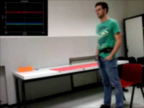## Video dataset overview Follow this link to see a video of the 6 activities recorded in the experiment with one of the participants:

[Watch video]

## Details about input data I will be using an LSTM on the data to learn (as a cellphone attached on the waist) to recognise the type of activity that the user is doing. The dataset's description goes like this: > The sensor signals (accelerometer and gyroscope) were pre-processed by applying noise filters and then sampled in fixed-width sliding windows of 2.56 sec and 50% overlap (128 readings/window). The sensor acceleration signal, which has gravitational and body motion components, was separated using a Butterworth low-pass filter into body acceleration and gravity. The gravitational force is assumed to have only low frequency components, therefore a filter with 0.3 Hz cutoff frequency was used. That said, I will use the almost raw data: only the gravity effect has been filtered out of the accelerometer as a preprocessing step for another 3D feature as an input to help learning. ## What is an RNN? 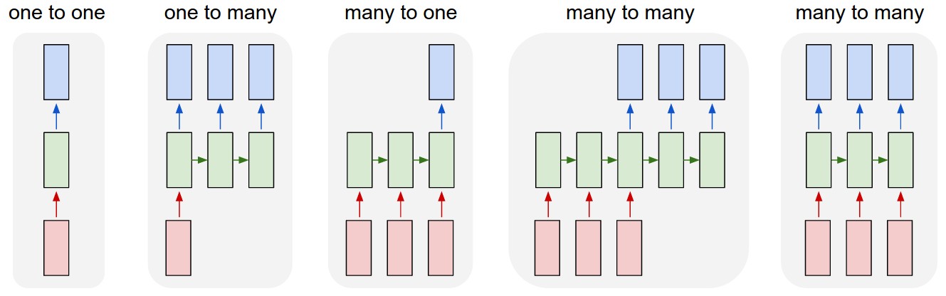As explained in [this article](http://karpathy.github.io/2015/05/21/rnn-effectiveness/), an RNN takes many input vectors to process them and output other vectors. It can be roughly pictured like in the image below, imagining each rectangle has a vectorial depth and other special hidden quirks in the image below. **In our case, the "many to one" architecture is used**: we accept time series of feature vectors (one vector per time step) to convert them to a probability vector at the output for classification. Note that a "one to one" architecture would be a standard feedforward neural network. An LSTM is an improved RNN. It is more complex, but easier to train, avoiding what is called the vanishing gradient problem. ## Results Scroll on! Nice visuals awaits. ```python # All Includes import numpy as np import matplotlib import matplotlib.pyplot as plt import tensorflow as tf # Version 1.0.0 (some previous versions are used in past commits) from sklearn import metrics import os ``` ```python # Useful Constants # Those are separate normalised input features for the neural network INPUT_SIGNAL_TYPES = [ "body_acc_x_", "body_acc_y_", "body_acc_z_", "body_gyro_x_", "body_gyro_y_", "body_gyro_z_", "total_acc_x_", "total_acc_y_", "total_acc_z_" ] # Output classes to learn how to classify LABELS = [ "WALKING", "WALKING_UPSTAIRS", "WALKING_DOWNSTAIRS", "SITTING", "STANDING", "LAYING" ] ``` ## Let's start by downloading the data: ```python # Note: Linux bash commands start with a "!" inside those "ipython notebook" cells DATA_PATH = "data/" !pwd && ls os.chdir(DATA_PATH) !pwd && ls !python download_dataset.py !pwd && ls os.chdir("..") !pwd && ls DATASET_PATH = DATA_PATH + "UCI HAR Dataset/" print("\n" + "Dataset is now located at: " + DATASET_PATH) ``` /home/ubuntu/pynb/LSTM-Human-Activity-Recognition data LSTM_files LSTM_OLD.ipynb README.md LICENSE LSTM.ipynb lstm.py screenlog.0 /home/ubuntu/pynb/LSTM-Human-Activity-Recognition/data download_dataset.py source.txt Downloading... --2017-05-24 01:49:53-- https://archive.ics.uci.edu/ml/machine-learning-databases/00240/UCI%20HAR%20Dataset.zip Resolving archive.ics.uci.edu (archive.ics.uci.edu)... 128.195.10.249 Connecting to archive.ics.uci.edu (archive.ics.uci.edu)|128.195.10.249|:443... connected. HTTP request sent, awaiting response... 200 OK Length: 60999314 (58M) [application/zip] Saving to: ‘UCI HAR Dataset.zip’ 100%[======================================>] 60,999,314 1.69MB/s in 38s 2017-05-24 01:50:31 (1.55 MB/s) - ‘UCI HAR Dataset.zip’ saved [60999314/60999314] Downloading done. Extracting... Extracting successfully done to /home/ubuntu/pynb/LSTM-Human-Activity-Recognition/data/UCI HAR Dataset. /home/ubuntu/pynb/LSTM-Human-Activity-Recognition/data download_dataset.py __MACOSX source.txt UCI HAR Dataset UCI HAR Dataset.zip /home/ubuntu/pynb/LSTM-Human-Activity-Recognition data LSTM_files LSTM_OLD.ipynb README.md LICENSE LSTM.ipynb lstm.py screenlog.0 Dataset is now located at: data/UCI HAR Dataset/ ## Preparing dataset: ```python TRAIN = "train/" TEST = "test/" # Load "X" (the neural network's training and testing inputs) def load_X(X_signals_paths): X_signals = [] for signal_type_path in X_signals_paths: file = open(signal_type_path, 'r') # Read dataset from disk, dealing with text files' syntax X_signals.append( [np.array(serie, dtype=np.float32) for serie in [ row.replace(' ', ' ').strip().split(' ') for row in file ]] ) file.close() return np.transpose(np.array(X_signals), (1, 2, 0)) X_train_signals_paths = [ DATASET_PATH + TRAIN + "Inertial Signals/" + signal + "train.txt" for signal in INPUT_SIGNAL_TYPES ] X_test_signals_paths = [ DATASET_PATH + TEST + "Inertial Signals/" + signal + "test.txt" for signal in INPUT_SIGNAL_TYPES ] X_train = load_X(X_train_signals_paths) X_test = load_X(X_test_signals_paths) # Load "y" (the neural network's training and testing outputs) def load_y(y_path): file = open(y_path, 'r') # Read dataset from disk, dealing with text file's syntax y_ = np.array( [elem for elem in [ row.replace(' ', ' ').strip().split(' ') for row in file ]], dtype=np.int32 ) file.close() # Substract 1 to each output class for friendly 0-based indexing return y_ - 1 y_train_path = DATASET_PATH + TRAIN + "y_train.txt" y_test_path = DATASET_PATH + TEST + "y_test.txt" y_train = load_y(y_train_path) y_test = load_y(y_test_path) ``` ## Additionnal Parameters: Here are some core parameter definitions for the training. The whole neural network's structure could be summarised by enumerating those parameters and the fact an LSTM is used. ```python # Input Data training_data_count = len(X_train) # 7352 training series (with 50% overlap between each serie) test_data_count = len(X_test) # 2947 testing series n_steps = len(X_train[0]) # 128 timesteps per series n_input = len(X_train[0][0]) # 9 input parameters per timestep # LSTM Neural Network's internal structure n_hidden = 32 # Hidden layer num of features n_classes = 6 # Total classes (should go up, or should go down) # Training learning_rate = 0.0025 lambda_loss_amount = 0.0015 training_iters = training_data_count * 300 # Loop 300 times on the dataset batch_size = 1500 display_iter = 30000 # To show test set accuracy during training # Some debugging info print("Some useful info to get an insight on dataset's shape and normalisation:") print("(X shape, y shape, every X's mean, every X's standard deviation)") print(X_test.shape, y_test.shape, np.mean(X_test), np.std(X_test)) print("The dataset is therefore properly normalised, as expected, but not yet one-hot encoded.") ``` Some useful info to get an insight on dataset's shape and normalisation: (X shape, y shape, every X's mean, every X's standard deviation) (2947, 128, 9) (2947, 1) 0.0991399 0.395671 The dataset is therefore properly normalised, as expected, but not yet one-hot encoded. ## Utility functions for training: ```python def LSTM_RNN(_X, _weights, _biases): # Function returns a tensorflow LSTM (RNN) artificial neural network from given parameters. # Moreover, two LSTM cells are stacked which adds deepness to the neural network. # Note, some code of this notebook is inspired from an slightly different # RNN architecture used on another dataset, some of the credits goes to # "aymericdamien" under the MIT license. # (NOTE: This step could be greatly optimised by shaping the dataset once # input shape: (batch_size, n_steps, n_input) _X = tf.transpose(_X, [1, 0, 2]) # permute n_steps and batch_size # Reshape to prepare input to hidden activation _X = tf.reshape(_X, [-1, n_input]) # new shape: (n_steps*batch_size, n_input) # Linear activation _X = tf.nn.relu(tf.matmul(_X, _weights['hidden']) + _biases['hidden']) # Split data because rnn cell needs a list of inputs for the RNN inner loop _X = tf.split(_X, n_steps, 0) # new shape: n_steps * (batch_size, n_hidden) # Define two stacked LSTM cells (two recurrent layers deep) with tensorflow lstm_cell_1 = tf.contrib.rnn.BasicLSTMCell(n_hidden, forget_bias=1.0, state_is_tuple=True) lstm_cell_2 = tf.contrib.rnn.BasicLSTMCell(n_hidden, forget_bias=1.0, state_is_tuple=True) lstm_cells = tf.contrib.rnn.MultiRNNCell([lstm_cell_1, lstm_cell_2], state_is_tuple=True) # Get LSTM cell output outputs, states = tf.contrib.rnn.static_rnn(lstm_cells, _X, dtype=tf.float32) # Get last time step's output feature for a "many to one" style classifier, # as in the image describing RNNs at the top of this page lstm_last_output = outputs[-1] # Linear activation return tf.matmul(lstm_last_output, _weights['out']) + _biases['out'] def extract_batch_size(_train, step, batch_size): # Function to fetch a "batch_size" amount of data from "(X|y)_train" data. shape = list(_train.shape) shape[0] = batch_size batch_s = np.empty(shape) for i in range(batch_size): # Loop index index = ((step-1)*batch_size + i) % len(_train) batch_s[i] = _train[index] return batch_s def one_hot(y_): # Function to encode output labels from number indexes # e.g.: [[5], [0], [3]] --> [[0, 0, 0, 0, 0, 1], [1, 0, 0, 0, 0, 0], [0, 0, 0, 1, 0, 0]] y_ = y_.reshape(len(y_)) n_values = int(np.max(y_)) + 1 return np.eye(n_values)[np.array(y_, dtype=np.int32)] # Returns FLOATS ``` ## Let's get serious and build the neural network: ```python # Graph input/output x = tf.placeholder(tf.float32, [None, n_steps, n_input]) y = tf.placeholder(tf.float32, [None, n_classes]) # Graph weights weights = { 'hidden': tf.Variable(tf.random_normal([n_input, n_hidden])), # Hidden layer weights 'out': tf.Variable(tf.random_normal([n_hidden, n_classes], mean=1.0)) } biases = { 'hidden': tf.Variable(tf.random_normal([n_hidden])), 'out': tf.Variable(tf.random_normal([n_classes])) } pred = LSTM_RNN(x, weights, biases) # Loss, optimizer and evaluation l2 = lambda_loss_amount * sum( tf.nn.l2_loss(tf_var) for tf_var in tf.trainable_variables() ) # L2 loss prevents this overkill neural network to overfit the data cost = tf.reduce_mean(tf.nn.softmax_cross_entropy_with_logits(labels=y, logits=pred)) + l2 # Softmax loss optimizer = tf.train.AdamOptimizer(learning_rate=learning_rate).minimize(cost) # Adam Optimizer correct_pred = tf.equal(tf.argmax(pred,1), tf.argmax(y,1)) accuracy = tf.reduce_mean(tf.cast(correct_pred, tf.float32)) ``` ## Hooray, now train the neural network: ```python # To keep track of training's performance test_losses = [] test_accuracies = [] train_losses = [] train_accuracies = [] # Launch the graph sess = tf.InteractiveSession(config=tf.ConfigProto(log_device_placement=True)) init = tf.global_variables_initializer() sess.run(init) # Perform Training steps with "batch_size" amount of example data at each loop step = 1 while step * batch_size <= training_iters: batch_xs = extract_batch_size(X_train, step, batch_size) batch_ys = one_hot(extract_batch_size(y_train, step, batch_size)) # Fit training using batch data _, loss, acc = sess.run( [optimizer, cost, accuracy], feed_dict={ x: batch_xs, y: batch_ys } ) train_losses.append(loss) train_accuracies.append(acc) # Evaluate network only at some steps for faster training: if (step*batch_size % display_iter == 0) or (step == 1) or (step * batch_size > training_iters): # To not spam console, show training accuracy/loss in this "if" print("Training iter #" + str(step*batch_size) + \ ": Batch Loss = " + "{:.6f}".format(loss) + \ ", Accuracy = {}".format(acc)) # Evaluation on the test set (no learning made here - just evaluation for diagnosis) loss, acc = sess.run( [cost, accuracy], feed_dict={ x: X_test, y: one_hot(y_test) } ) test_losses.append(loss) test_accuracies.append(acc) print("PERFORMANCE ON TEST SET: " + \ "Batch Loss = {}".format(loss) + \ ", Accuracy = {}".format(acc)) step += 1 print("Optimization Finished!") # Accuracy for test data one_hot_predictions, accuracy, final_loss = sess.run( [pred, accuracy, cost], feed_dict={ x: X_test, y: one_hot(y_test) } ) test_losses.append(final_loss) test_accuracies.append(accuracy) print("FINAL RESULT: " + \ "Batch Loss = {}".format(final_loss) + \ ", Accuracy = {}".format(accuracy)) ``` WARNING:tensorflow:From :9: initialize_all_variables (from tensorflow.python.ops.variables) is deprecated and will be removed after 2017-03-02. Instructions for updating: Use `tf.global_variables_initializer` instead. Training iter #1500: Batch Loss = 5.416760, Accuracy = 0.15266665816307068 PERFORMANCE ON TEST SET: Batch Loss = 4.88082***11096191, Accuracy = 0.056328471750020*** Training iter #30000: Batch Loss = 3.031930, Accuracy = 0.607333242893219 PERFORMANCE ON TEST SET: Batch Loss = 3.0515167713165283, Accuracy = 0.6067186594009399 Training iter #60000: Batch Loss = 2.6727***, Accuracy = 0.7386666536331177 PERFORMANCE ON TEST SET: Batch Loss = 2.780435085296631, Accuracy = 0.7027485370635***6 Training iter #90000: Batch Loss = 2.378301, Accuracy = 0.8366667032241821 PERFORMANCE ON TEST SET: Batch Loss = 2.6019773483276367, Accuracy = 0.7617915868759155 Training iter #120000: Batch Loss = 2.127290, Accuracy = 0.9066667556762695 PERFORMANCE ON TEST SET: Batch Loss = 2.3625404834747314, Accuracy = 0.8116728663444519 Training iter #150000: Batch Loss = 1.92***05, Accuracy = 0.9380000233650208 PERFORMANCE ON TEST SET: Batch Loss = 2.306251049041748, Accuracy = 0.8276212215423584 Training iter #180000: Batch Loss = 1.971904, Accuracy = 0.9153333902359009 PERFORMANCE ON TEST SET: Batch Loss = 2.0835530757904053, Accuracy = 0.8771631121635437 Training iter #210000: Batch Loss = 1.860249, Accuracy = 0.8613333702087402 PERFORMANCE ON TEST SET: Batch Loss = 1.9994492530822754, Accuracy = 0.8788597583770752 Training iter #240000: Batch Loss = 1.626292, Accuracy = 0.9380000233650208 PERFORMANCE ON TEST SET: Batch Loss = 1.879166603088379, Accuracy = 0.8944689035415***9 Training iter #270000: Batch Loss = 1.582758, Accuracy = 0.9386667013168335 PERFORMANCE ON TEST SET: Batch Loss = 2.0341007709503174, Accuracy = 0.8361043930053711 Training iter #300000: Batch Loss = 1.620352, Accuracy = 0.9306666851043701 PERFORMANCE ON TEST SET: Batch Loss = 1.8185184001922607, Accuracy = 0.863929331302***28 Training iter #330000: Batch Loss = 1.474394, Accuracy = 0.9693333506584167 PERFORMANCE ON TEST SET: Batch Loss = 1.76385033130***575, Accuracy = 0.8747878670692444 Training iter #360000: Batch Loss = 1.4069***, Accuracy = 0.9420000314712524 PERFORMANCE ON TEST SET: Batch Loss = 1.5946787595748901, Accuracy = 0.902273416519165 Training iter #390000: Batch Loss = 1.362515, Accuracy = 0.940000057220459 PERFORMANCE ON TEST SET: Batch Loss = 1.5285792350769043, Accuracy = 0.904***87212181091 Training iter #420000: Batch Loss = 1.252860, Accuracy = 0.9566667079925537 PERFORMANCE ON TEST SET: Batch Loss = 1.4635565280914307, Accuracy = 0.910756587***21777 Training iter #450000: Batch Loss = 1.190078, Accuracy = 0.9553333520889282 PERFORMANCE ON TEST SET: Batch Loss = 1.442753553390503, Accuracy = 0.9093992710113525 Training iter #480000: Batch Loss = 1.159610, Accuracy = 0.9446667432785034 PERFORMANCE ON TEST SET: Batch Loss = 1.4130011796951294, Accuracy = 0.8971834778785706 Training iter #510000: Batch Loss = 1.100551, Accuracy = 0.9593333601951599 PERFORMANCE ON TEST SET: Batch Loss = 1.3075592517852783, Accuracy = 0.9117745757102966 Training iter #540000: Batch Loss = 1.123470, Accuracy = 0.9240000247955322 PERFORMANCE ON TEST SET: Batch Loss = 1.2605488300323486, Accuracy = 0.9165251851081848 Training iter #570000: Batch Loss = 1.103454, Accuracy = 0.909333348274231 PERFORMANCE ON TEST SET: Batch Loss = 1.2327136993408203, Accuracy = 0.9009160399436951 Training iter #600000: Batch Loss = 1.083368, Accuracy = 0.896666***60037231 PERFORMANCE ON TEST SET: Batch Loss = 1.2683708667755127, Accuracy = 0.88903951***489746 Training iter #630000: Batch Loss = 0.939185, Accuracy = 0.9700000882148743 PERFORMANCE ON TEST SET: Batch Loss = 1.2147629261016846, Accuracy = 0.8866***2713546753 Training iter #660000: Batch Loss = 0.881242, Accuracy = 0.***06667566299438 PERFORMANCE ON TEST SET: Batch Loss = 1.1068334579467773, Accuracy = 0.9151678681373596 Training iter #690000: Batch Loss = 0.831674, Accuracy = 0.***5333442687***83 PERFORMANCE ON TEST SET: Batch Loss = 1.0885852575302124, Accuracy = 0.9121139***557***77 Training iter #720000: Batch Loss = 0.866615, Accuracy = 0.9573334455490112 PERFORMANCE ON TEST SET: Batch Loss = 1.05135166***505005, Accuracy = 0.9158465266227722 Training iter #750000: Batch Loss = 0.858979, Accuracy = 0.940000057220459 PERFORMANCE ON TEST SET: Batch Loss = 1.05***633289337158, Accuracy = 0.906345367431***06 Training iter #780000: Batch Loss = 0.750040, Accuracy = 0.95933341979***047 PERFORMANCE ON TEST SET: Batch Loss = 1.01096***20173***5, Accuracy = 0.9155071973800659 Training iter #810000: Batch Loss = 0.732136, Accuracy = 0.9620000123977661 PERFORMANCE ON TEST SET: Batch Loss = 0.***6569***30206299, Accuracy = 0.9161 ... ...

近期下载者：

相关文件：

评论：[我要评论] [举报此文件]

收藏者：