CliqueNet-master
说明: achieve image classificaition using clique
文件列表:
LICENSE (1066, 2018-06-15)
dataloader (0, 2018-06-15)
dataloader\__init__.py (0, 2018-06-15)
dataloader\data_generator.py (3993, 2018-06-15)
dataloader\preprocess.py (3442, 2018-06-15)
imagenet_pytorch (0, 2018-06-15)
imagenet_pytorch\__init__.py (0, 2018-06-15)
imagenet_pytorch\cliquenet.py (3569, 2018-06-15)
imagenet_pytorch\utils.py (8322, 2018-06-15)
img (0, 2018-06-15)
img\fig1.JPG (40419, 2018-06-15)
img\fig2.JPG (78275, 2018-06-15)
img\fig3.JPG (28630, 2018-06-15)
img\tab1.JPG (70226, 2018-06-15)
models (0, 2018-06-15)
models\__init__.py (0, 2018-06-15)
models\cliquenet.py (1568, 2018-06-15)
models\cliquenet_I_I.py (1572, 2018-06-15)
models\cliquenet_I_II.py (1573, 2018-06-15)
models\cliquenet_X.py (1578, 2018-06-15)
models\utils.py (22126, 2018-06-15)
train.py (7870, 2018-06-15)
train_imagenet.py (10381, 2018-06-15)
# CliqueNet
This repository is for [Convolutional Neural Networks with Alternately Updated Clique](https://arxiv.org/abs/1802.10419) (to appear in CVPR 2018, Oral presentation),
by Yibo Yang, Zhisheng Zhong, Tiancheng Shen, and [Zhouchen Lin](http://www.cis.pku.edu.cn/faculty/vision/zlin/zlin.htm).
### citation
If you find CliqueNet useful in your research, please consider citing:
@article{yang18,
author={Yibo Yang and Zhisheng Zhong and Tiancheng Shen and Zhouchen Lin},
title={Convolutional Neural Networks with Alternately Updated Clique},
journal={arXiv preprint arXiv:1802.10419},
year={2018}
}
### table of contents
- [Introduction](#introduction)
- [Usage](#usage)
- [Ablation experiments](#ablation-experiments)
- [Comparison with state of the arts](#comparision-with-state-of-the-arts)
- [Results on ImageNet](#results-on-imagenet)
## Introduction
CliqueNet is a newly proposed convolutional neural network architecture where any pair of layers in the same block are connected bilaterally (Fig 1). Any layer is both the input and output another one, and information flow can be maximized. During propagation, the layers are updated alternately (Fig 2), so that each layer will always receive the feedback information from the layers that are updated more lately. We show that the refined features are more discriminative and lead to a better performance. On benchmark classification datasets including CIFAR-10, CIFAR-100, SVHN, and ILSVRC 2012, we achieve better or comparable results over state of the arts with fewer parameters. This repo contains the code of our project, and also provides some experimental results that are out of the paper.
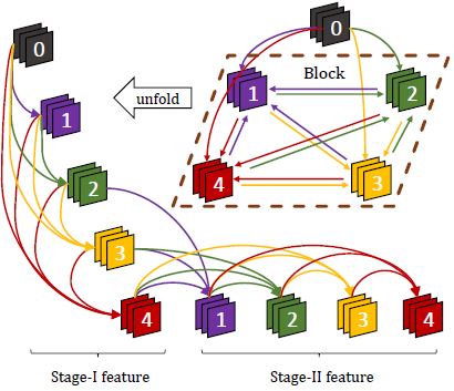 Fig 1. An illustration of a block with 4 layers. Node 0 denotes the input layer of this block.
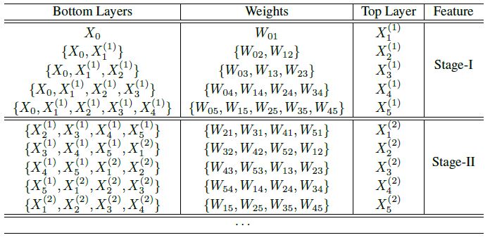 Fig 2. Alternate updating rule in CliqueNet. "{}" denotes the concatenating operator.
## Usage
- Our experiments are conducted with [TensorFlow](https://github.com/tensorflow/tensorflow) in Python 2.
- Clone this repo: `git clone https://github.com/iboing/CliqueNet`
- An example to train a model on CIFAR or SVHN:
```bash
python train.py --gpu [gpu id] --dataset [cifar-10 or cifar-100 or SVHN] --k [filters per layer] --T [all layers of three blocks] --dir [path to save models]
```
- Additional techniques (optional): if you want to use attentional transition, bottleneck architecture, or compression strategy in our paper, add `--if_a True`, `--if_b True`, and `--if_c True`, respectively.
## Ablation experiments
With the feedback connections, CliqueNet alternately re-update previous layers with updated layers, to enable refined features. The weights among layers are re-used for multiple times, so that a deeper representation space can be attained with a fixed number of parameters. In order to test the effectiveness of CliqueNet's feature refinement, we analyze the features generated in different stages by conducting experiments using different versions of CliqueNet. As illustrated by Fig 3, the CliqueNet(I+I) only uses Stage-I feature. The CliqueNet(I+II) uses Stage-I feature concatenated with input layer as the block feature, but transits Stage-II feature into the next block. The CliqueNet(II+II) only uses refined features.
Fig 2. Alternate updating rule in CliqueNet. "{}" denotes the concatenating operator.
## Usage
- Our experiments are conducted with [TensorFlow](https://github.com/tensorflow/tensorflow) in Python 2.
- Clone this repo: `git clone https://github.com/iboing/CliqueNet`
- An example to train a model on CIFAR or SVHN:
```bash
python train.py --gpu [gpu id] --dataset [cifar-10 or cifar-100 or SVHN] --k [filters per layer] --T [all layers of three blocks] --dir [path to save models]
```
- Additional techniques (optional): if you want to use attentional transition, bottleneck architecture, or compression strategy in our paper, add `--if_a True`, `--if_b True`, and `--if_c True`, respectively.
## Ablation experiments
With the feedback connections, CliqueNet alternately re-update previous layers with updated layers, to enable refined features. The weights among layers are re-used for multiple times, so that a deeper representation space can be attained with a fixed number of parameters. In order to test the effectiveness of CliqueNet's feature refinement, we analyze the features generated in different stages by conducting experiments using different versions of CliqueNet. As illustrated by Fig 3, the CliqueNet(I+I) only uses Stage-I feature. The CliqueNet(I+II) uses Stage-I feature concatenated with input layer as the block feature, but transits Stage-II feature into the next block. The CliqueNet(II+II) only uses refined features.
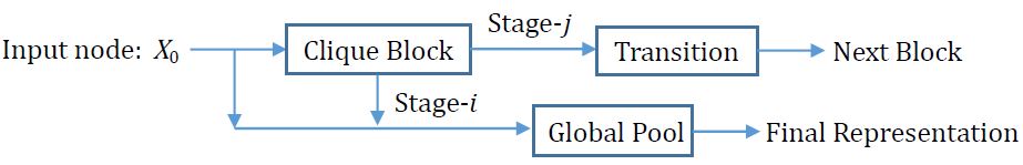 Fig 3. A schema for CliqueNet(i+j), i,j belong to {I,II}.
|Model |block feature |transit |error(%)|
|-----------------|-----------------|--------|--------|
|CliqueNet(I+I) |{ X_0, Stage-I } |Stage-I |6.*** |
|CliqueNet(I+II) |{ X_0, Stage-I } |Stage-II|6.10 |
|CliqueNet(II+II) |{ X_0, Stage-II }|Stage-II|5.76 |
Tab 1. Resutls of different versions of CliqueNets.
To run the experiments above, please modify `train.py` as:
```python
from models.cliquenet_I_I import build_model
```
for CliqueNet(I+I), and
```python
from models.cliquenet_I_II import build_model
```
for CliqueNet(I+II).
We further consider a situation where the feedback is not processed entirely. Concretely, when k=*** and T=15, we use the Stage-II feature, but only the first `X` steps, see Fig 2. Then `X=0` is just the case of CliqueNet(I+I), and `X=5` corresponds to CliqueNet(II+II).
|Model|CIFAR-10| CIFAR-100|
|--------------|----|-----|
|CliqueNet(X=0)|5.83|24.79|
|CliqueNet(X=1)|5.63|24.65|
|CliqueNet(X=2)|5.54|24.37|
|CliqueNet(X=3)|5.41|23.75|
|CliqueNet(X=4)|5.20|24.04|
|CliqueNet(X=5)|5.12|23.73|
Tab 2. Performance of CliqueNets with different `X`.
To run the experiments with different `X`, modify `train.py` as:
```python
from models.cliquenet_X import build_model
```
and set the value of `X` in `./models/cliquenet_X.py`
## Comparison with state of the arts
The results listed below demonstrate the superiority of CliqueNet over DenseNet when there are no additional techniques (bottleneck, compression, etc.).
|Model | FLOPs | Params | CIFAR-10 | CIFAR-100 | SVHN |
|------------------------------------| ------|--------| -------- |-----------|------|
|DenseNet (k = 12, T = 36) | 0.53G | 1.0M | 7.00 | 27.55 | 1.79 |
|DenseNet (k = 12, T = 96) | 3.54G | 7.0M | 5.77 | 23.79 | 1.67 |
|DenseNet (k = 24, T = 96) | 13.78G| 27.2M | 5.83 | 23.42 | 1.59 |
| | | | | | |
|CliqueNet (k = 36, T = 12) | 0.91G | 0.94M | 5.93 | 27.32 | 1.77 |
|CliqueNet (k = ***, T = 15) | 4.21G | 4.49M | 5.12 | 23.*** | 1.62 |
|CliqueNet (k = 80, T = 15) | ***5G | 6.94M | 5.10 | 23.32 | 1.56 |
|CliqueNet (k = 80, T = 18) | 9.45G | 10.14M | 5.06 | 23.14 | 1.51 |
Tab 3. Main results on CIFAR and SVHN without data augmentation.
Because larger T would lead to higher computation cost and slightly more parameters, we prefer using a larger k in our experiments. To make comparisons more fair, we also consider the situation where k and T of DenseNets and CliqueNets are exactly the same, see Tab 4.
|Model|Params|CIFAR-10 | CIFAR-100|
|--------------------|-----|----|-----|
|DenseNet(k=12,T=36) |1.02M|7.00|27.55|
|CliqueNet(k=12,T=36)|1.05M|5.79|26.85|
| | | | |
|DenseNet(k=24,T=18) |0.99M|7.13|27.70|
|CliqueNet(k=24,T=18)|0.99M|6.04|26.57|
| | | | |
|DenseNet(k=36,T=12) |0.96M|6.89|27.54|
|CliqueNet(k=36,T=12)|0.94M|5.93|27.32|
Tab 4. Comparisons with the same k and T.
Note that the result of DenseNet(k=12, T=36) is reported by original paper. The others are implementated by ourselves under the same experimental settings.
## Results on ImageNet
Our code for experiments on ImageNet with TensorFlow will be released soon.
Here we provide a [PyTorch](http://pytorch.org) version to train a CliqueNet on ImageNet. An example to run:
```Python
python train_imagenet.py [path to the imagenet dataset]
```
(As the default, CliqueNet-S3 is trained, batchsize is 160 and attentional transition is used.)
The PyTorch pre-trained model can be downloaded here (Google Drive): [S3_model](https://drive.google.com/file/d/1fvaSSiy590reWK0a0mNSJqmkr4yCqpI-/view?usp=sharing).
Fig 3. A schema for CliqueNet(i+j), i,j belong to {I,II}.
|Model |block feature |transit |error(%)|
|-----------------|-----------------|--------|--------|
|CliqueNet(I+I) |{ X_0, Stage-I } |Stage-I |6.*** |
|CliqueNet(I+II) |{ X_0, Stage-I } |Stage-II|6.10 |
|CliqueNet(II+II) |{ X_0, Stage-II }|Stage-II|5.76 |
Tab 1. Resutls of different versions of CliqueNets.
To run the experiments above, please modify `train.py` as:
```python
from models.cliquenet_I_I import build_model
```
for CliqueNet(I+I), and
```python
from models.cliquenet_I_II import build_model
```
for CliqueNet(I+II).
We further consider a situation where the feedback is not processed entirely. Concretely, when k=*** and T=15, we use the Stage-II feature, but only the first `X` steps, see Fig 2. Then `X=0` is just the case of CliqueNet(I+I), and `X=5` corresponds to CliqueNet(II+II).
|Model|CIFAR-10| CIFAR-100|
|--------------|----|-----|
|CliqueNet(X=0)|5.83|24.79|
|CliqueNet(X=1)|5.63|24.65|
|CliqueNet(X=2)|5.54|24.37|
|CliqueNet(X=3)|5.41|23.75|
|CliqueNet(X=4)|5.20|24.04|
|CliqueNet(X=5)|5.12|23.73|
Tab 2. Performance of CliqueNets with different `X`.
To run the experiments with different `X`, modify `train.py` as:
```python
from models.cliquenet_X import build_model
```
and set the value of `X` in `./models/cliquenet_X.py`
## Comparison with state of the arts
The results listed below demonstrate the superiority of CliqueNet over DenseNet when there are no additional techniques (bottleneck, compression, etc.).
|Model | FLOPs | Params | CIFAR-10 | CIFAR-100 | SVHN |
|------------------------------------| ------|--------| -------- |-----------|------|
|DenseNet (k = 12, T = 36) | 0.53G | 1.0M | 7.00 | 27.55 | 1.79 |
|DenseNet (k = 12, T = 96) | 3.54G | 7.0M | 5.77 | 23.79 | 1.67 |
|DenseNet (k = 24, T = 96) | 13.78G| 27.2M | 5.83 | 23.42 | 1.59 |
| | | | | | |
|CliqueNet (k = 36, T = 12) | 0.91G | 0.94M | 5.93 | 27.32 | 1.77 |
|CliqueNet (k = ***, T = 15) | 4.21G | 4.49M | 5.12 | 23.*** | 1.62 |
|CliqueNet (k = 80, T = 15) | ***5G | 6.94M | 5.10 | 23.32 | 1.56 |
|CliqueNet (k = 80, T = 18) | 9.45G | 10.14M | 5.06 | 23.14 | 1.51 |
Tab 3. Main results on CIFAR and SVHN without data augmentation.
Because larger T would lead to higher computation cost and slightly more parameters, we prefer using a larger k in our experiments. To make comparisons more fair, we also consider the situation where k and T of DenseNets and CliqueNets are exactly the same, see Tab 4.
|Model|Params|CIFAR-10 | CIFAR-100|
|--------------------|-----|----|-----|
|DenseNet(k=12,T=36) |1.02M|7.00|27.55|
|CliqueNet(k=12,T=36)|1.05M|5.79|26.85|
| | | | |
|DenseNet(k=24,T=18) |0.99M|7.13|27.70|
|CliqueNet(k=24,T=18)|0.99M|6.04|26.57|
| | | | |
|DenseNet(k=36,T=12) |0.96M|6.89|27.54|
|CliqueNet(k=36,T=12)|0.94M|5.93|27.32|
Tab 4. Comparisons with the same k and T.
Note that the result of DenseNet(k=12, T=36) is reported by original paper. The others are implementated by ourselves under the same experimental settings.
## Results on ImageNet
Our code for experiments on ImageNet with TensorFlow will be released soon.
Here we provide a [PyTorch](http://pytorch.org) version to train a CliqueNet on ImageNet. An example to run:
```Python
python train_imagenet.py [path to the imagenet dataset]
```
(As the default, CliqueNet-S3 is trained, batchsize is 160 and attentional transition is used.)
The PyTorch pre-trained model can be downloaded here (Google Drive): [S3_model](https://drive.google.com/file/d/1fvaSSiy590reWK0a0mNSJqmkr4yCqpI-/view?usp=sharing).
Fig 1. An illustration of a block with 4 layers. Node 0 denotes the input layer of this block.
Fig 2. Alternate updating rule in CliqueNet. "{}" denotes the concatenating operator.
## Usage
- Our experiments are conducted with [TensorFlow](https://github.com/tensorflow/tensorflow) in Python 2.
- Clone this repo: `git clone https://github.com/iboing/CliqueNet`
- An example to train a model on CIFAR or SVHN:
```bash
python train.py --gpu [gpu id] --dataset [cifar-10 or cifar-100 or SVHN] --k [filters per layer] --T [all layers of three blocks] --dir [path to save models]
```
- Additional techniques (optional): if you want to use attentional transition, bottleneck architecture, or compression strategy in our paper, add `--if_a True`, `--if_b True`, and `--if_c True`, respectively.
## Ablation experiments
With the feedback connections, CliqueNet alternately re-update previous layers with updated layers, to enable refined features. The weights among layers are re-used for multiple times, so that a deeper representation space can be attained with a fixed number of parameters. In order to test the effectiveness of CliqueNet's feature refinement, we analyze the features generated in different stages by conducting experiments using different versions of CliqueNet. As illustrated by Fig 3, the CliqueNet(I+I) only uses Stage-I feature. The CliqueNet(I+II) uses Stage-I feature concatenated with input layer as the block feature, but transits Stage-II feature into the next block. The CliqueNet(II+II) only uses refined features.
Fig 3. A schema for CliqueNet(i+j), i,j belong to {I,II}.
|Model |block feature |transit |error(%)|
|-----------------|-----------------|--------|--------|
|CliqueNet(I+I) |{ X_0, Stage-I } |Stage-I |6.*** |
|CliqueNet(I+II) |{ X_0, Stage-I } |Stage-II|6.10 |
|CliqueNet(II+II) |{ X_0, Stage-II }|Stage-II|5.76 |
Tab 1. Resutls of different versions of CliqueNets.
To run the experiments above, please modify `train.py` as:
```python
from models.cliquenet_I_I import build_model
```
for CliqueNet(I+I), and
```python
from models.cliquenet_I_II import build_model
```
for CliqueNet(I+II).
We further consider a situation where the feedback is not processed entirely. Concretely, when k=*** and T=15, we use the Stage-II feature, but only the first `X` steps, see Fig 2. Then `X=0` is just the case of CliqueNet(I+I), and `X=5` corresponds to CliqueNet(II+II).
|Model|CIFAR-10| CIFAR-100|
|--------------|----|-----|
|CliqueNet(X=0)|5.83|24.79|
|CliqueNet(X=1)|5.63|24.65|
|CliqueNet(X=2)|5.54|24.37|
|CliqueNet(X=3)|5.41|23.75|
|CliqueNet(X=4)|5.20|24.04|
|CliqueNet(X=5)|5.12|23.73|
Tab 2. Performance of CliqueNets with different `X`.
To run the experiments with different `X`, modify `train.py` as:
```python
from models.cliquenet_X import build_model
```
and set the value of `X` in `./models/cliquenet_X.py`
## Comparison with state of the arts
The results listed below demonstrate the superiority of CliqueNet over DenseNet when there are no additional techniques (bottleneck, compression, etc.).
|Model | FLOPs | Params | CIFAR-10 | CIFAR-100 | SVHN |
|------------------------------------| ------|--------| -------- |-----------|------|
|DenseNet (k = 12, T = 36) | 0.53G | 1.0M | 7.00 | 27.55 | 1.79 |
|DenseNet (k = 12, T = 96) | 3.54G | 7.0M | 5.77 | 23.79 | 1.67 |
|DenseNet (k = 24, T = 96) | 13.78G| 27.2M | 5.83 | 23.42 | 1.59 |
| | | | | | |
|CliqueNet (k = 36, T = 12) | 0.91G | 0.94M | 5.93 | 27.32 | 1.77 |
|CliqueNet (k = ***, T = 15) | 4.21G | 4.49M | 5.12 | 23.*** | 1.62 |
|CliqueNet (k = 80, T = 15) | ***5G | 6.94M | 5.10 | 23.32 | 1.56 |
|CliqueNet (k = 80, T = 18) | 9.45G | 10.14M | 5.06 | 23.14 | 1.51 |
Tab 3. Main results on CIFAR and SVHN without data augmentation.
Because larger T would lead to higher computation cost and slightly more parameters, we prefer using a larger k in our experiments. To make comparisons more fair, we also consider the situation where k and T of DenseNets and CliqueNets are exactly the same, see Tab 4.
|Model|Params|CIFAR-10 | CIFAR-100|
|--------------------|-----|----|-----|
|DenseNet(k=12,T=36) |1.02M|7.00|27.55|
|CliqueNet(k=12,T=36)|1.05M|5.79|26.85|
| | | | |
|DenseNet(k=24,T=18) |0.99M|7.13|27.70|
|CliqueNet(k=24,T=18)|0.99M|6.04|26.57|
| | | | |
|DenseNet(k=36,T=12) |0.96M|6.89|27.54|
|CliqueNet(k=36,T=12)|0.94M|5.93|27.32|
Tab 4. Comparisons with the same k and T.
Note that the result of DenseNet(k=12, T=36) is reported by original paper. The others are implementated by ourselves under the same experimental settings.
## Results on ImageNet
Our code for experiments on ImageNet with TensorFlow will be released soon.
Here we provide a [PyTorch](http://pytorch.org) version to train a CliqueNet on ImageNet. An example to run:
```Python
python train_imagenet.py [path to the imagenet dataset]
```
(As the default, CliqueNet-S3 is trained, batchsize is 160 and attentional transition is used.)
The PyTorch pre-trained model can be downloaded here (Google Drive): [S3_model](https://drive.google.com/file/d/1fvaSSiy590reWK0a0mNSJqmkr4yCqpI-/view?usp=sharing).
近期下载者:
相关文件:
收藏者: