文件列表:

LICENSE (1086, 2019-12-09)
LSTM.ipynb (213539, 2019-12-09)
LSTM_files (0, 2019-12-09)
LSTM_files\LSTM_16_0.png (77480, 2019-12-09)
LSTM_files\LSTM_18_1.png (43286, 2019-12-09)
data (0, 2019-12-09)
data\download_dataset.py (914, 2019-12-09)
data\source.txt (2068, 2019-12-09)

# LSTMs for Human Activity Recognition Human Activity Recognition (HAR) using smartphones dataset and an LSTM RNN. Classifying the type of movement amongst six categories: - WALKING, - WALKING_UPSTAIRS, - WALKING_DOWNSTAIRS, - SITTING, - STANDING, - LAYING. Compared to a classical approach, using a Recurrent Neural Networks (RNN) with Long Short-Term Memory cells (LSTMs) require no or almost no feature engineering. Data can be fed directly into the neural network who acts like a black box, modeling the problem correctly. [Other research](https://archive.ics.uci.edu/ml/machine-learning-databases/00240/UCI%20HAR%20Dataset.names) on the activity recognition dataset can use a big amount of feature engineering, which is rather a signal processing approach combined with classical data science techniques. The approach here is rather very simple in terms of how much was the data preprocessed. Let's use Google's neat Deep Learning library, TensorFlow, demonstrating the usage of an LSTM, a type of Artificial Neural Network that can process sequential data / time series. ## Video dataset overview Follow this link to see a video of the 6 activities recorded in the experiment with one of the participants:

[Watch video]

## Details about the input data I will be using an LSTM on the data to learn (as a cellphone attached on the waist) to recognise the type of activity that the user is doing. The dataset's description goes like this: > The sensor signals (accelerometer and gyroscope) were pre-processed by applying noise filters and then sampled in fixed-width sliding windows of 2.56 sec and 50% overlap (128 readings/window). The sensor acceleration signal, which has gravitational and body motion components, was separated using a Butterworth low-pass filter into body acceleration and gravity. The gravitational force is assumed to have only low frequency components, therefore a filter with 0.3 Hz cutoff frequency was used. That said, I will use the almost raw data: only the gravity effect has been filtered out of the accelerometer as a preprocessing step for another 3D feature as an input to help learning. If you'd ever want to extract the gravity by yourself, you could fork my code on using a [Butterworth Low-Pass Filter (LPF) in Python](https://github.com/guillaume-chevalier/filtering-stft-and-laplace-transform) and edit it to have the right cutoff frequency of 0.3 Hz which is a good frequency for activity recognition from body sensors. ## What is an RNN? 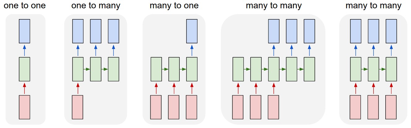As explained in [this article](http://karpathy.github.io/2015/05/21/rnn-effectiveness/), an RNN takes many input vectors to process them and output other vectors. It can be roughly pictured like in the image below, imagining each rectangle has a vectorial depth and other special hidden quirks in the image below. **In our case, the "many to one" architecture is used**: we accept time series of [feature vectors](https://www.quora.com/What-do-samples-features-time-steps-mean-in-LSTM/answer/Guillaume-Chevalier-2) (one vector per [time step](https://www.quora.com/What-do-samples-features-time-steps-mean-in-LSTM/answer/Guillaume-Chevalier-2)) to convert them to a probability vector at the output for classification. Note that a "one to one" architecture would be a standard feedforward neural network. > > http://karpathy.github.io/2015/05/21/rnn-effectiveness/ ## What is an LSTM? An LSTM is an improved RNN. It is more complex, but easier to train, avoiding what is called the vanishing gradient problem. I recommend [this article](http://colah.github.io/posts/2015-08-Understanding-LSTMs/) for you to learn more on LSTMs. ## Results Scroll on! Nice visuals awaits. ```python # All Includes import numpy as np import matplotlib import matplotlib.pyplot as plt import tensorflow as tf # Version 1.0.0 (some previous versions are used in past commits) from sklearn import metrics import os ``` ```python # Useful Constants # Those are separate normalised input features for the neural network INPUT_SIGNAL_TYPES = [ "body_acc_x_", "body_acc_y_", "body_acc_z_", "body_gyro_x_", "body_gyro_y_", "body_gyro_z_", "total_acc_x_", "total_acc_y_", "total_acc_z_" ] # Output classes to learn how to classify LABELS = [ "WALKING", "WALKING_UPSTAIRS", "WALKING_DOWNSTAIRS", "SITTING", "STANDING", "LAYING" ] ``` ## Let's start by downloading the data: ```python # Note: Linux bash commands start with a "!" inside those "ipython notebook" cells DATA_PATH = "data/" !pwd && ls os.chdir(DATA_PATH) !pwd && ls !python download_dataset.py !pwd && ls os.chdir("..") !pwd && ls DATASET_PATH = DATA_PATH + "UCI HAR Dataset/" print("\n" + "Dataset is now located at: " + DATASET_PATH) ``` /home/ubuntu/pynb/LSTM-Human-Activity-Recognition data LSTM_files LSTM_OLD.ipynb README.md LICENSE LSTM.ipynb lstm.py screenlog.0 /home/ubuntu/pynb/LSTM-Human-Activity-Recognition/data download_dataset.py source.txt Downloading... --2017-05-24 01:49:53-- https://archive.ics.uci.edu/ml/machine-learning-databases/00240/UCI%20HAR%20Dataset.zip Resolving archive.ics.uci.edu (archive.ics.uci.edu)... 128.195.10.249 Connecting to archive.ics.uci.edu (archive.ics.uci.edu)|128.195.10.249|:443... connected. HTTP request sent, awaiting response... 200 OK Length: 60999314 (58M) [application/zip] Saving to: ‘UCI HAR Dataset.zip’ 100%[======================================>] 60,999,314 1.69MB/s in 38s 2017-05-24 01:50:31 (1.55 MB/s) - ‘UCI HAR Dataset.zip’ saved [60999314/60999314] Downloading done. Extracting... Extracting successfully done to /home/ubuntu/pynb/LSTM-Human-Activity-Recognition/data/UCI HAR Dataset. /home/ubuntu/pynb/LSTM-Human-Activity-Recognition/data download_dataset.py __MACOSX source.txt UCI HAR Dataset UCI HAR Dataset.zip /home/ubuntu/pynb/LSTM-Human-Activity-Recognition data LSTM_files LSTM_OLD.ipynb README.md LICENSE LSTM.ipynb lstm.py screenlog.0 Dataset is now located at: data/UCI HAR Dataset/ ## Preparing dataset: ```python TRAIN = "train/" TEST = "test/" # Load "X" (the neural network's training and testing inputs) def load_X(X_signals_paths): X_signals = [] for signal_type_path in X_signals_paths: file = open(signal_type_path, 'r') # Read dataset from disk, dealing with text files' syntax X_signals.append( [np.array(serie, dtype=np.float32) for serie in [ row.replace(' ', ' ').strip().split(' ') for row in file ]] ) file.close() return np.transpose(np.array(X_signals), (1, 2, 0)) X_train_signals_paths = [ DATASET_PATH + TRAIN + "Inertial Signals/" + signal + "train.txt" for signal in INPUT_SIGNAL_TYPES ] X_test_signals_paths = [ DATASET_PATH + TEST + "Inertial Signals/" + signal + "test.txt" for signal in INPUT_SIGNAL_TYPES ] X_train = load_X(X_train_signals_paths) X_test = load_X(X_test_signals_paths) # Load "y" (the neural network's training and testing outputs) def load_y(y_path): file = open(y_path, 'r') # Read dataset from disk, dealing with text file's syntax y_ = np.array( [elem for elem in [ row.replace(' ', ' ').strip().split(' ') for row in file ]], dtype=np.int32 ) file.close() # Substract 1 to each output class for friendly 0-based indexing return y_ - 1 y_train_path = DATASET_PATH + TRAIN + "y_train.txt" y_test_path = DATASET_PATH + TEST + "y_test.txt" y_train = load_y(y_train_path) y_test = load_y(y_test_path) ``` ## Additionnal Parameters: Here are some core parameter definitions for the training. For example, the whole neural network's structure could be summarised by enumerating those parameters and the fact that two LSTM are used one on top of another (stacked) output-to-input as hidden layers through time steps. ```python # Input Data training_data_count = len(X_train) # 7352 training series (with 50% overlap between each serie) test_data_count = len(X_test) # 2947 testing series n_steps = len(X_train[0]) # 128 timesteps per series n_input = len(X_train[0][0]) # 9 input parameters per timestep # LSTM Neural Network's internal structure n_hidden = 32 # Hidden layer num of features n_classes = 6 # Total classes (should go up, or should go down) # Training learning_rate = 0.0025 lambda_loss_amount = 0.0015 training_iters = training_data_count * 300 # Loop 300 times on the dataset batch_size = 1500 display_iter = 30000 # To show test set accuracy during training # Some debugging info print("Some useful info to get an insight on dataset's shape and normalisation:") print("(X shape, y shape, every X's mean, every X's standard deviation)") print(X_test.shape, y_test.shape, np.mean(X_test), np.std(X_test)) print("The dataset is therefore properly normalised, as expected, but not yet one-hot encoded.") ``` Some useful info to get an insight on dataset's shape and normalisation: (X shape, y shape, every X's mean, every X's standard deviation) (2947, 128, 9) (2947, 1) 0.0991399 0.395671 The dataset is therefore properly normalised, as expected, but not yet one-hot encoded. ## Utility functions for training: ```python def LSTM_RNN(_X, _weights, _biases): # Function returns a tensorflow LSTM (RNN) artificial neural network from given parameters. # Moreover, two LSTM cells are stacked which adds deepness to the neural network. # Note, some code of this notebook is inspired from an slightly different # RNN architecture used on another dataset, some of the credits goes to # "aymericdamien" under the MIT license. # (NOTE: This step could be greatly optimised by shaping the dataset once # input shape: (batch_size, n_steps, n_input) _X = tf.transpose(_X, [1, 0, 2]) # permute n_steps and batch_size # Reshape to prepare input to hidden activation _X = tf.reshape(_X, [-1, n_input]) # new shape: (n_steps*batch_size, n_input) # ReLU activation, thanks to Yu Zhao for adding this improvement here: _X = tf.nn.relu(tf.matmul(_X, _weights['hidden']) + _biases['hidden']) # Split data because rnn cell needs a list of inputs for the RNN inner loop _X = tf.split(_X, n_steps, 0) # new shape: n_steps * (batch_size, n_hidden) # Define two stacked LSTM cells (two recurrent layers deep) with tensorflow lstm_cell_1 = tf.contrib.rnn.BasicLSTMCell(n_hidden, forget_bias=1.0, state_is_tuple=True) lstm_cell_2 = tf.contrib.rnn.BasicLSTMCell(n_hidden, forget_bias=1.0, state_is_tuple=True) lstm_cells = tf.contrib.rnn.MultiRNNCell([lstm_cell_1, lstm_cell_2], state_is_tuple=True) # Get LSTM cell output outputs, states = tf.contrib.rnn.static_rnn(lstm_cells, _X, dtype=tf.float32) # Get last time step's output feature for a "many-to-one" style classifier, # as in the image describing RNNs at the top of this page lstm_last_output = outputs[-1] # Linear activation return tf.matmul(lstm_last_output, _weights['out']) + _biases['out'] def extract_batch_size(_train, step, batch_size): # Function to fetch a "batch_size" amount of data from "(X|y)_train" data. shape = list(_train.shape) shape[0] = batch_size batch_s = np.empty(shape) for i in range(batch_size): # Loop index index = ((step-1)*batch_size + i) % len(_train) batch_s[i] = _train[index] return batch_s def one_hot(y_, n_classes=n_classes): # Function to encode neural one-hot output labels from number indexes # e.g.: # one_hot(y_=[[5], [0], [3]], n_classes=6): # return [[0, 0, 0, 0, 0, 1], [1, 0, 0, 0, 0, 0], [0, 0, 0, 1, 0, 0]] y_ = y_.reshape(len(y_)) return np.eye(n_classes)[np.array(y_, dtype=np.int32)] # Returns FLOATS ``` ## Let's get serious and build the neural network: ```python # Graph input/output x = tf.placeholder(tf.float32, [None, n_steps, n_input]) y = tf.placeholder(tf.float32, [None, n_classes]) # Graph weights weights = { 'hidden': tf.Variable(tf.random_normal([n_input, n_hidden])), # Hidden layer weights 'out': tf.Variable(tf.random_normal([n_hidden, n_classes], mean=1.0)) } biases = { 'hidden': tf.Variable(tf.random_normal([n_hidden])), 'out': tf.Variable(tf.random_normal([n_classes])) } pred = LSTM_RNN(x, weights, biases) # Loss, optimizer and evaluation l2 = lambda_loss_amount * sum( tf.nn.l2_loss(tf_var) for tf_var in tf.trainable_variables() ) # L2 loss prevents this overkill neural network to overfit the data cost = tf.reduce_mean(tf.nn.softmax_cross_entropy_with_logits(labels=y, logits=pred)) + l2 # Softmax loss optimizer = tf.train.AdamOptimizer(learning_rate=learning_rate).minimize(cost) # Adam Optimizer correct_pred = tf.equal(tf.argmax(pred,1), tf.argmax(y,1)) accuracy = tf.reduce_mean(tf.cast(correct_pred, tf.float32)) ``` ## Hooray, now train the neural network: ```python # To keep track of training's performance test_losses = [] test_accuracies = [] train_losses = [] train_accuracies = [] # Launch the graph sess = tf.InteractiveSession(config=tf.ConfigProto(log_device_placement=True)) init = tf.global_variables_initializer() sess.run(init) # Perform Training steps with "batch_size" amount of example data at each loop step = 1 while step * batch_size <= training_iters: batch_xs = extract_batch_size(X_train, step, batch_size) batch_ys = one_hot(extract_batch_size(y_train, step, batch_size)) # Fit training using batch data _, loss, acc = sess.run( [optimizer, cost, accuracy], feed_dict={ x: batch_xs, y: batch_ys } ) train_losses.append(loss) train_accuracies.append(acc) # Evaluate network only at some steps for faster training: if (step*batch_size % display_iter == 0) or (step == 1) or (step * batch_size > training_iters): # To not spam console, show training accuracy/loss in this "if" print("Training iter #" + str(step*batch_size) + \ ": Batch Loss = " + "{:.6f}".format(loss) + \ ", Accuracy = {}".format(acc)) # Evaluation on the test set (no learning made here - just evaluation for diagnosis) loss, acc = sess.run( [cost, accuracy], feed_dict={ x: X_test, y: one_hot(y_test) } ) test_losses.append(loss) test_accuracies.append(acc) print("PERFORMANCE ON TEST SET: " + \ "Batch Loss = {}".format(loss) + \ ", Accuracy = {}".format(acc)) step += 1 print("Optimization Finished!") # Accuracy for test data one_hot_predictions, accuracy, final_loss = sess.run( [pred, accuracy, cost], feed_dict={ x: X_test, y: one_hot(y_test) } ) test_losses.append(final_loss) test_accuracies.append(accuracy) print("FINAL RESULT: " + \ "Batch Loss = {}".format(final_loss) + \ ", Accuracy = {}".format(accuracy)) ``` WARNING:tensorflow:From :9: initialize_all_variables (from tensorflow.python.ops.variables) is deprecated and will be removed after 2017-03-02. Instructions for updating: Use `tf.global_variables_initializer` instead. Training iter #1500: Batch Loss = 5.416760, Accuracy = 0.15266665816307068 PERFORMANCE ON TEST SET: Batch Loss = 4.88082***11096191, Accuracy = 0.056328471750020*** Training iter #30000: Batch Loss = 3.031930, Accuracy = 0.607333242893219 PERFORMANCE ON TEST SET: Batch Loss = 3.0515167713165283, Accuracy = 0.6067186594009399 Training iter #60000: Batch Loss = 2.6727***, Accuracy = 0.7386666536331177 PERFORMANCE ON TEST SET: Batch Loss = 2.780435085296631, Accuracy = 0.7027485370635***6 Training iter #90000: Batch Loss = 2.378301, Accuracy = 0.8366667032241821 PERFORMANCE ON TEST SET: Batch Loss = 2.6019773483276367, Accuracy = 0.7617915868759155 Training iter #120000: Batch Loss = 2.127290, Accuracy = 0.9066667556762695 PERFORMANCE ON TEST SET: Batch Loss = 2.3625404834747314, Accuracy = 0.8116728663444519 Training iter #150000: Batch Loss = 1.92***05, Accuracy = 0.9380000233650208 PERFORMANCE ON TEST SET: Batch Loss = 2.306251049041748, Accuracy = 0.8276212215423584 Training iter #180000: Batch Loss = 1.971904, Accuracy = 0.9153333902359009 PERFORMANCE ON TEST SET: Batch Loss = 2.0835530757904053, Accuracy = 0.8771631121635437 Training iter #210000: Batch Loss = 1.860249, Accuracy = 0.8613333702087402 PERFORMANCE ON TEST SET: Batch Loss = 1.9994492530822754, Accuracy = 0.8788597583770752 Training iter #240000: Batch Loss = 1.626292, Accuracy = 0.9380000233650208 PERFORMANCE ON TEST SET: Batch Loss = 1.879166603088379, Accuracy = 0.8944689035415***9 Training iter #270000: Batch Loss = 1.582758, Accuracy = 0.9386667013168335 PERFORMANCE ON TEST SET: Batch Loss = 2.0341007709503174, Accuracy = 0.8361043930053711 Training iter #300000: Batch Loss = 1.620352, Accuracy = 0.9306666851043701 PERFORMANCE ON TEST SET: Batch Loss = 1.8185184001922607, Accuracy = 0.863929331302***28 Training iter #330000: Batch Loss = 1.474394, Accuracy = 0.9693333506584167 PERFORMANCE ON TEST SET: Batch Loss = 1.76385033130***575, Accuracy = 0.8747878670692444 Training iter #360000: Batch Loss = 1.4069***, Accuracy = 0.9420000314712524 PERFORMANCE ON TEST SET: Batch Loss = 1.5946787595748901, Accuracy = 0.902273416519165 Training iter #390000: Batch Loss = 1.362515, Accuracy = 0.940000057220459 PERFORMANCE ON TEST SET: Batch Loss = 1.5285792350769043, Accuracy = 0.904***87212181091 Training iter #420000: Batch Loss = 1.252860, Accuracy = 0.9566667079925537 PERFORMANCE ON TEST SET: Batch Loss = 1.4635565280914307, Accuracy = 0.910756587***21777 Training iter #450000: Batch Loss = 1.190078, Accuracy = 0.9553333520889282 ... PERFORMANCE ON TEST SET: Batch Loss = 0.425678***060401917, Accuracy = 0.9324736595153809 Training iter #2070000: Batch Loss = 0.342763, Accuracy = 0.93266671895***083 PERFORMANCE ON TEST SET: Batch Loss = 0.4292***3412742615, Accuracy = 0.9273836612701416 Training iter #2100000: Batch Loss = 0.259442, Accuracy = 0.***73334169387817 PERFORMANCE ON TEST SET: Batch Loss = 0.44131210446357727, Accuracy = 0.9273836612701416 Training iter #2130000: Batch Loss = 0.284630, Accuracy = 0.9593333601951599 PERFORMANCE ON TEST SET: Batch Loss = 0.46***2717514038086, Accuracy = 0.9093992710113525 Training iter #2160000: Batch Loss = 0.299012, Accuracy = 0.9686667323112488 PERFORMANCE ON TEST SET: Batch Loss = 0.48389002680778503, Accuracy = 0.9138105511665344 Training iter #2190000: Batch Loss = 0.287106, Accuracy = 0.97000002861022 ... ...

近期下载者：

相关文件：

评论：[我要评论] [举报此文件]

收藏者：