文件列表:

.travis.yml (90, 2018-04-08)
DESCRIPTION (1090, 2018-04-08)
NAMESPACE (323, 2018-04-08)
R (0, 2018-04-08)
R\robspca.R (11306, 2018-04-08)
R\rspca.R (12202, 2018-04-08)
R\spca.R (10537, 2018-04-08)
man (0, 2018-04-08)
man\robspca.Rd (4517, 2018-04-08)
man\rspca.Rd (5252, 2018-04-08)
man\spca.Rd (4103, 2018-04-08)
plots (0, 2018-04-08)
plots\eigenfaces.png (234796, 2018-04-08)
plots\objective.svg (30259, 2018-04-08)
plots\robustsparseeigenfaces.png (84987, 2018-04-08)
plots\sparsecomp.png (8475, 2018-04-08)
plots\sparseeigenfaces.png (87117, 2018-04-08)
plots\sparsereigenfaces.png (49421, 2018-04-08)
plots\timeing.png (7408, 2018-04-08)
plots\timeing_art.png (7808, 2018-04-08)
spca.png (45195, 2018-04-08)
tests (0, 2018-04-08)
tests\testthat (0, 2018-04-08)
tests\testthat\test_robspca.R (3508, 2018-04-08)
tests\testthat\test_rspca.R (3221, 2018-04-08)
tests\testthat\test_spca.R (3212, 2018-04-08)

[](https://travis-ci.org/erichson/spca) # SPCA via Variable Projection Sparse principal component analysis (SPCA) is a modern variant of PCA. Specifically, SPCA attempts to find sparse weight vectors (loadings), i.e., a weight vector with only a few `active' (nonzero) values. This approach leads to an improved interpretability of the model, because the principal components are formed as a linear combination of only a few of the original variables. Further, SPCA avoids overfitting in a high-dimensional data setting where the number of variables is greater than the number of observations. This package provides robust and randomized accelerated SPCA routines in R: * Sparse PCA: ``spca()``. * Randomized SPCA: ``rspca()``. * Robust SPCA: ``robspca()``. ## Problem Formulation Such a parsimonious model is obtained by introducing prior information like sparsity promoting regularizers. More concreatly, given a data matrix ``X`` with shape ``(m,p)``, SPCA attemps to minimize the following optimization problem: ``` minimize f(A,B) = 1/2‖X - XBAT‖2 + α‖B‖1 + 1/2β‖B‖2, subject to ATA = I. ``` The matrix ``B`` is the sparse weight (loadings) matrix and ``A`` is an orthonormal matrix. Here we use a combination of the l1 and l2 norm as a sparsity-promoting regularizer, also known as the elastic net. Then, the principal components ``Z`` are then formed as ``` Z = X %*% B. ``` Specifically, the interface of the SPCA function is: ```R spca(X, k, alpha=1e-4, beta=1e-4, center=TRUE, scale=TRUE, max_iter=1000, tol=1e-4, verbose=TRUE) ``` The description of the arguments is listed in the following: * ``X`` is a real ``n`` by ``p`` data matrix (or data frame), where ``n`` denotes the number of observations and ``p`` the number of variables. * ``k`` specifies the target rank, i.e., number of components to be computed. * ``alpha`` is a sparsity controlling parameter. Higher values lead to sparser components. * `` beta`` controls the amount of ridge shrinkage to apply in order to improve conditioning. * ``center`` logical value which indicates whether the variables should be shifted to be zero centered (TRUE by default). * ``scale``logical value which indicates whether the variables should be scaled to have unit variance (FALSE by default). * ``max_iter`` maximum number of iterations to perform before exiting. * ``tol`` stopping tolerance for reconstruction error. * ``verbose`` logical value which indicates whether progress is printed. A list with the following components is returned: * ``loadings`` sparse loadings (weight) vector. * ``transform`` the approximated inverse transform to rotate the scores back to high-dimensional space. * ``scores`` the principal component scores. * ``eigenvalues`` the approximated eigenvalues; * ``center, scale`` the centering and scaling used. ## Installation Install the sparsepca package via CRAN ```R install.packages("sparsepca") ``` You can also install the development version from GitHub using [devtools](https://cran.r-project.org/package=devtools): ```r devtools::install_github("erichson/spca") ``` ## Example: Sparse PCA One of the most striking demonstrations of PCA are eigenfaces. The aim is to extract the most dominant correlations between different faces from a large set of facial images. Specifically, the resulting columns of the rotation matrix (i.e., the eigenvectors) represent `shadows' of the faces, the so-called eigenfaces. Specifically, the eigenfaces reveal both inner face features (e.g., eyes, nose, mouth) and outer features (e.g., head shape, hairline, eyebrows). These features can then be used for facial recognition and classification. In the following we use the down-sampled cropped Yale face database B. The dataset comprises 2410 grayscale images of 38 different people, cropped and aligned, and can be loaded as ```r utils::download.file('https://github.com/erichson/data/blob/master/R/faces.RData?raw=true', 'faces.RData', "wget") load("faces.RData") ``` For computational convenience the 96x84 faces images are stored as column vectors of the data matrix. For instance, the first face can be displayed as ```r face <- matrix(rev(faces[ , 1]), nrow = 84, ncol = 96) image(face, col = gray(0:255 / 255)) ``` In order to approximate the ``k=25`` dominant eigenfaces you can use the standard PCA function in R: ```r faces.pca <- prcomp(t(faces), k = 25, center = TRUE, scale. = TRUE) ``` Note, that the data matrix needs to be transposed, so that each column corresponds to a pixel location rather than to a person. Here, the analysis is performed on the correlation matrix by setting the argument \code{scale = TRUE}. The mean face is provided as the attribute ``center``. In the following, we use the SPCA package: ```r library("spca") ``` First, we set the tuning parameters ``alpha=0`` and ``beta=0``, which reduces to PCA: ```r spca.results <- spca(t(faces), k=25, alpha=0, beta=0, center=TRUE, scale=TRUE) ``` The summary of the analysis is as follows: ```r summary(spca.results) PC1 PC2 PC3 PC4 PC5 ... Explained variance 2901.541 2706.701 388.080 227.062 118.407 ... Standard deviations 53.866 52.026 19.700 15.069 10.882 ... Proportion of variance 0.360 0.336 0.048 0.028 0.015 ... Cumulative proportion 0.360 0.695 0.744 0.772 0.786 ... 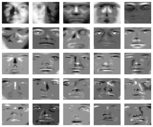``` Just the first 5 PCs explain about 79% of the total variation in the data, while the first 25 PCs explain more then 90%. Finally, the eigenvectors can be visualized as eigenfaces, e.g., the first eigenvector (eigenface) is displayed as follows ```r layout(matrix(1:25, 5, 5, byrow = TRUE)) for(i in 1:25) { par(mar = c(0.5,0.5,0.5,0.5)) img <- matrix(spca.results$loadings[,i], nrow=84, ncol=96) image(img[,96:1], col = gray((255:0)/255), axes=FALSE, xaxs="i", yaxs="i", xaxt='n', yaxt='n',ann=FALSE ) } ``` The eigenfaces encode the holistic facial features as well as the illumination. In many application, however, it is favorable to obtain a sparse representation. This is because a sparse representation is easier to interpret. Further, this avoids overfitting in a high-dimensional data setting where the number of variables is greater than the number of observations. SPCA attempts to find sparse weight vectors (loadings), i.e., the approximate eigenvecotrs with only a few `active' (nonzero) values. We can compute the sparse eigenvectors as follows: ```r rspca.results <- rspca(t(faces), k=25, alpha=1e-4, beta=1e-1, verbose=1, max_iter=1000, tol=1e-4, center=TRUE, scale=TRUE) ``` the objective values for each iteration can be plotted as: ```r plot(log(rspca.results$objective), col='red', xlab='Number of iterations', ylab='Objective value') ``` Note, that we have use here the randomized accelerated SPCA algorithm! The randomized algorithm eases the computational demands and is suitable if the input data feature some low-rank structure. For more details about randomized methods see, for instance, [Randomized Matrix Decompositions using R](http://arxiv.org/abs/1608.02148). Now, ``summary(rspca.results)`` reveals that the first 5 PCs only explain about 67% of the total variation. However, we yield a parsimonious representation of the data: ```r layout(matrix(1:25, 5, 5, byrow = TRUE)) for(i in 1:25) { par(mar = c(0.5,0.5,0.5,0.5)) img <- matrix(rspca.results$loadings[,i], nrow=84, ncol=96) image(img[,96:1], col = gray((255:0)/255), axes=FALSE, xaxs="i", yaxs="i", xaxt='n', yaxt='n',ann=FALSE ) } ``` Unlike PCA, the sparse loadings contextualize localized features. If desired the solution can be made even sparser by increasing the tuning parameter ``alpha``: ```r rspca.results <- rspca(t(faces), k=25, alpha=2e-4, beta=2e-1, verbose=1, max_iter=1000, tol=1e-4, center=TRUE, scale=TRUE) ``` We yield the following sparse loadings: ```r layout(matrix(1:25, 5, 5, byrow = TRUE)) for(i in 1:25) { par(mar = c(0.5,0.5,0.5,0.5)) img <- matrix(rspca.results$loadings[,i], nrow=84, ncol=96) image(img[,96:1], col = gray((255:0)/255), axes=FALSE, xaxs="i", yaxs="i", xaxt='n', yaxt='n',ann=FALSE ) } ``` ## Computational Comparison Now, let us evaluate the computatinal performace. Here we consider for comparision also the SPCA function from the ``elasticnet`` package. First, we create some artificial data where we know the ground truth: ```r m <- 100000 V1 <- rnorm(m, 0, 290) V2 <- rnorm(m, 0, 300) V3 <- -0.1*V1 + 0.1*V2 + rnorm(m,0,100) X <- cbind(V1,V1,V1,V1, V2,V2,V2,V2, V3,V3) X <- X + matrix(rnorm(length(X),0,1), ncol = ncol(X), nrow = nrow(X)) ``` Hence, we expect to find 3 components. The first and second should have 4 non-zero loadings and the third 2 non-zero loadings. As a sanity check you can plot the loadings: ```r out <- rspca(X, k=3, alpha=1e-4, beta=1e-4, center = TRUE, scale = FALSE, verbose=0) print(out) Standard deviations: [1] 599.686 578.621 137.740 Eigenvalues: [1] 359623.56 334802.29 18972.17 Sparse loadings: [,1] [,2] [,3] [1,] 0.000 -0.4*** 0.000 [2,] 0.000 -0.4*** 0.000 [3,] 0.000 -0.4*** 0.000 [4,] 0.000 -0.4*** 0.000 [5,] -0.499 0.000 0.000 [6,] -0.499 0.000 0.000 [7,] -0.499 0.000 0.000 [8,] -0.499 0.000 0.000 [9,] 0.000 0.000 0.678 [10,] 0.000 0.000 0.678 ``` Next, we use the ``microbenchmark`` package for timing: ```r library("microbenchmark") timing_spca = microbenchmark( 'Elastinet SPCA' = elasticnet::spca(X, K = 3, type = "predictor", sparse = "varnum", para = c(4, 4, 2)), 'Deterministic SPCA' = spca(X, k=3, alpha=1e-4, beta=1e-4, verbose=0), 'Randomized SPCA' = rspca(X, k=3, alpha=1e-4, beta=1e-4, verbose=0, o=0, q=0), times = 20 ) autoplot(timing_spca, log = TRUE, y_max = 1.05 * max(timing_spca$time)) ``` The performance is summarized in the following plot. 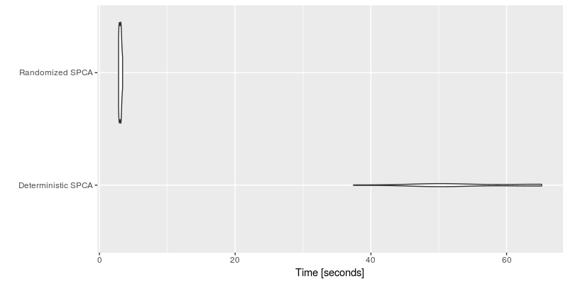We clearly see the computational advantage of the SPCA algorithm using variable projection compare to the implementation provided by the elastinet package. Further, we see that there is little difference between the randomized and the deterministic algorithms here. However, the performance is pronaunced for bigger datasets such as the face data. ```r timing_spca = microbenchmark( 'Deterministic SPCA' = spca(t(faces), k=25, alpha=1e-4, beta=1e-1, verbose=0, max_iter=1000, tol=1e-4), 'Randomized SPCA' = rspca(t(faces), k=25, alpha=1e-4, beta=1e-1, verbose=0, max_iter=1000, tol=1e-4), times = 15 ) autoplot(timing_spca, log = FALSE, y_max = 1.2 * max(timing_spca$time)) ``` Clearly, the randomized algorithm shows some substantial speedups over the deterministic algorithm. ## Example: Robust SPCA In the following we demonstrate the robust SCPA which allows to capture some grossly corrupted entries in the data. The idea is to separate the input data into a low-rank component and a sparse component. The latter aims to capture potential outliers in the data. For the face data, we proceed as follows: ```r robspca.results <- robspca(t(faces), k=25, alpha=1e-4, beta=1e-2, gamma=0.9, verbose=1, max_iter=1000, tol=1e-4, center=TRUE, scale=TRUE) ``` The tuning parameter ``gamma`` is the sparsity controlling parameter for the sparse error matrix. Smaller values lead to a larger amount of noise removeal. We yield the following sparse loadings: ```r layout(matrix(1:25, 5, 5, byrow = TRUE)) for(i in 1:25) { par(mar = c(0.5,0.5,0.5,0.5)) img <- matrix(robspca.results$loadings[,i], nrow=84, ncol=96) image(img[,96:1], col = gray((255:0)/255), axes=FALSE, xaxs="i", yaxs="i", xaxt='n', yaxt='n',ann=FALSE ) } ``` Further, we can visualize the captured outliers for each face. Here we show the outliers for the first 25 faces: ```r layout(matrix(1:25, 5, 5, byrow = TRUE)) for(i in 1:25) { par(mar = c(0.5,0.5,0.5,0.5)) img <- matrix(robspca.results$sparse[i,], nrow=84, ncol=96) image(img[,96:1], col = gray((255:0)/255), axes=FALSE, xaxs="i", yaxs="i", xaxt='n', yaxt='n',ann=FALSE ) } ``` 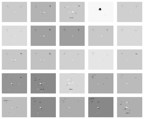It can be seen that the robust SPCA algorithms captures some of the specularities and other errors in the data. ## References * [N. Benjamin Erichson, et al. "Sparse Principal Component Analysis via Variable Projection." (2018)](https://arxiv.org/abs/1804.00341) * [N. Benjamin Erichson, et al. "Randomized Matrix Decompositions using R." (2016)](http://arxiv.org/abs/1608.02148)

近期下载者：

相关文件：

评论：[我要评论] [举报此文件]

收藏者：