文件列表:

PE.m (5112, 2018-10-22)
PE.png (55097, 2018-10-22)
_config.yml (26, 2018-10-22)
license.txt (1319, 2018-10-22)
table1.mat (180, 2018-10-22)
table2.mat (188, 2018-10-22)
table3.mat (211, 2018-10-22)
table4.mat (346, 2018-10-22)
table5.mat (1413, 2018-10-22)
table6.mat (9067, 2018-10-22)
table7.mat (73454, 2018-10-22)
table8.mat (854193, 2018-10-22)

# Fast-permutation-entropy Efficiently computing values of permutation entropy from 1D time series in sliding windows  function outdata = PE( indata, delay, order, windowSize ) computes efficiently [1] values of permutation entropy [2] for orders=1...8 of ordinal patterns from 1D time series in sliding windows. See more ordinal-patterns based measures at www.mathworks.com/matlabcentral/fileexchange/63782-ordinal-patterns-based-analysis--beta-version- NOTES - Order of ordinal patterns is defined as in [1,3,7,8], i.e. order = n-1 for n defined as in [2] - The values of permutation entropy are normalised by log((order+1)!) so that they are from [0,1] as proposed in the original paper [2]. INPUT - indata - 1D time series (1 x N points) - delay - delay between points in ordinal patterns (delay = 1 means successive points) - order - order of the ordinal patterns (order + 1 is the number of points in ordinal patterns) - windowSize - size of sliding window ( = number of ordinal patterns within sliding window) OUTPUT - outdata - (1 x (N - windowSize - order * delay) values of permutation entropy within [0,1] since each sliding window contains windowSize ordinal patterns but uses in fact (windowSize + order * delay + 1) points). 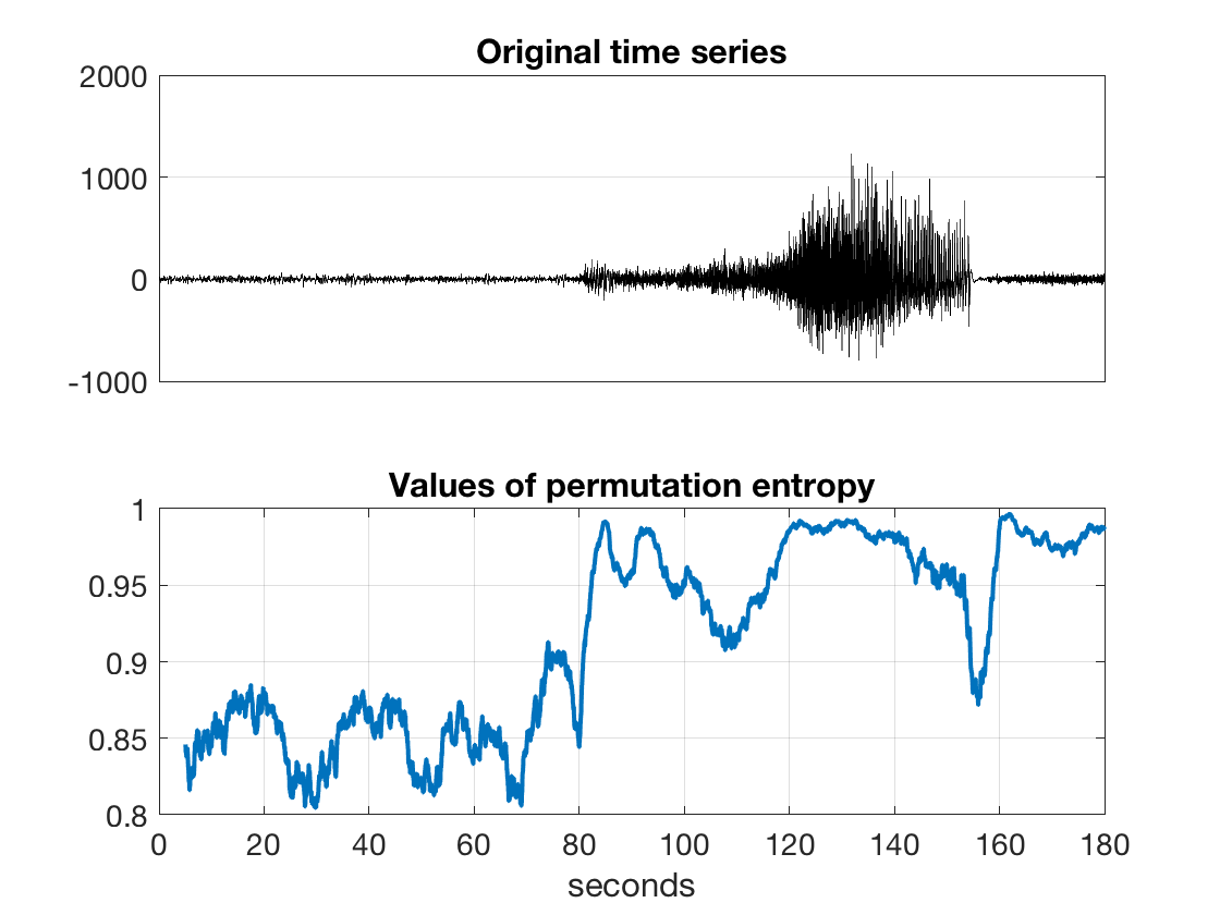INTERPRETATION The larger the values of permutation entropy (in the range from 0 to 1) are, the higher diversity of ordinal patterns is and the more complex input data are. CITING THE CODE - Unakafova, V.A., Keller, K., 2013. Efficiently measuring complexity on the basis of real-world data. Entropy, 15(10), 4392-4415. - Unakafova, Valentina (2015). Fast permutation entropy (www.mathworks.com/matlabcentral/fileexchange/44161-permutation-entropy--fast-algorithm-), MATLAB Central File Exchange. Retrieved Month Day, Year. EXAMPLE OF USE (with a plot): indata = rand( 1, 7777 ); % generate random data points for i = 4000:7000 % generate change of data complexity indata( i ) = 4 * indata( i - 1 )*( 1 - indata( i - 1 ) ); end delay = 1; % delay 1 between points in ordinal patterns (successive points) order = 3; % order 3 of ordinal patterns (4-points ordinal patterns) windowSize = 512; % 512 ordinal patterns in one sliding window outdata = PE( indata, delay, order, windowSize ); figure; ax1 = subplot( 2, 1, 1 ); plot( indata, 'k', 'LineWidth', 0.2 ); grid on; title( 'Original time series' ); ax2 = subplot( 2, 1, 2 ); plot( length(indata) - length(outdata)+1:length(indata), outdata, 'k', 'LineWidth', 0.2 ); grid on; title( 'Values of permutation entropy' ); linkaxes( [ ax1, ax2 ], 'x' ); CHOICE OF ORDER OF ORDINAL PATTERNS The larger order of ordinal patterns is, the better permutation entropy estimates complexity of the underlying dynamical system [3]. But for time series of finite length too large order of ordinal patterns leads to an underestimation of the complexity because not all ordinal patterns representing the system can occur [3]. Therefore, for practical applications, orders = 3...7 are often used [2,4,5,8]. In [6] the following rule for choice of order is recommended: 5*(order + 1)! < windowSize. CHOICE OF SLIDING WINDOW LENGTH Window size should be chosen in such way that time series is stationary within the window (for example, for EEG analysis 2 seconds sliding windows are often used) so that distribution of ordinal patterns would not change within the window [2,8], [3,Section 2.2], [7,Section 5.1.2]. CHOICE OF DELAY BETWEEN POINTS IN ORDINAL PATTERNS I would recommend choosing different delays and comparing results (see, for example, [3, Section 2.2-2.4] and [7, Chapter 5] for more details) though delay = 1 is often used for practical applications. Choice of delay depends on particular data analysis you perform [3,4], on type of pre-processing and on sampling rate of the data. For example, if you are interested in low-frequency part of signals it makes sense to use larger delays. REFERENCES [1] Unakafova, V.A., Keller, K., 2013. Efficiently measuring complexity on the basis of real-world Data. Entropy, 15(10), 4392-4415. [2] Bandt, C. and Pompe, B., 2002. Permutation entropy: a natural complexity measure for time series. Physical review letters, 88(17), p.174102. [3] Keller, K., Unakafov, A.M. and Unakafova, V.A., 2014. Ordinal patterns, entropy, and EEG. Entropy, 16(12), pp.6212-6239. [4] Riedl, M., Muller, A. and Wessel, N., 2013. Practical considerations of permutation entropy. The European Physical Journal Special Topics, 222(2), pp.249-262. [5] Zanin, M., Zunino, L., Rosso, O.A. and Papo, D., 2012. Permutation entropy and its main biomedical and econophysics applications: a review. Entropy, 14(8), pp.1553-1577. [6] Amigo, J.M., Zambrano, S. and Sanjuan, M.A., 2008. Combinatorial detection of determinism in noisy time series. EPL (Europhysics Letters), 83(6), p.60005. [7] Unakafova, V.A., 2015. Investigating measures of complexity for dynamical systems and for time series (Doctoral dissertation, University of Luebeck). [8] Keller, K., and M. Sinn. Ordinal analysis of time series. Physica A: Statistical Mechanics and its Applications 356.1 (2005): 114”120

近期下载者：

相关文件：

评论：[我要评论] [举报此文件]

收藏者：